Power log distributions
Central limit theorem
Suppose {X1, X2, …} is a sequence of i.i.d. random variables with $ E[X_i] = \mu $ and $ Var(X_i) = \sigma^2 $. Let $ S_n = \frac{X_1 + X_2 + .... + X_n}{n}$. Then, $ S_n \to N(\mu, \sigma^2 / n) $
Power log distribution
$ P[X = x] = C x^{- \alpha} \quad \quad x > x_{min} $
where,
$ C = (\alpha - 1) x_{min}^{(\alpha - 1)} $ and $ \alpha > 1 $
What's weird about Power log distributions?
Q1. What happens to expectation when $\alpha < 2$ ?
Q2. What happens to variance when $ \alpha < 3$ ?
Maximum Likelihood Estimation
Intuition:
- You are given a biased coin with probability p. You toss the coin a 100 times and observe 80 heads. Guess the value of p.
- Mathematically you can formulate the above problem as $$ p^* = argmax_{p} \; P[ \# \; heads = 80] $$
- Now,
$$ P[ \# \; heads = 80] = p^{80} . (1 - p)^{20} $$
- Differentiate wrt p to obtain p = 0.8
- This process is called maximum likelihood estimation. $ p ^ * $ is called the maximum likelihood estimate.
- We try to find the parameter of the distribution such that the Probability of observed values is maximised.
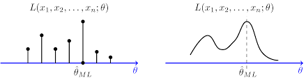
Locate the MLE from the figure
Exercise problems:
- Suppose you conduct a binomial experiment (Remember that a single binomial experiment consists of n iid Bernoulli experiments) with n = 10. Now you observe 7 heads and 3 tails in 10 tosses of the coin. Assume that the data comes from $ Binomial(10, p) $. Find the MLE of p.
- Now suppose you conduct three binomial experiments. You observe 7 heads 3 tails in exp 1, 6 heads 4 tails in exp 2, 8 heads 2 tails in exp 3. Again, assume that the data comes from $ Binomial(10, p)$. Find the MLE of p.
- Generalise: You conduct $ N $ number of $ Binomial(n, p) $ experiments, where $ n $ is known. You observe $ h_i $ heads in experiment i where i = 1, 2, 3 ... N. Find the MLE estimate of p.
What's good about MLE
- Intuitive.
- Point estimate: makes the math simple.
- As the number of samples increase, the estimate gets better. Mathematically, it achieves the Cramer - Rao bound
What's bad about MLE
- Point estimate: No knowledge about the confidence in the estimate.
- Can result in biased estimates
import matplotlib.pyplot as plt
%matplotlib inline
import numpy as np

p = np.arange(0, 1, 1/2000)
L = (p**8) * ((1-p)**2)
plt.plot(p, L)
plt.show()

L = (p**800) * ((1-p)**200)
plt.plot(p, L)


Bias and Variance of estimators
Wikipedia: https://en.wikipedia.org/wiki/Bias_of_an_estimator
Definition:
Suppose we have a statistical model, parameterized by a real number ''θ'', giving rise to a probability distribution for observed data, $ P_\theta(X) = P(X\mid\theta) $, and a statistic $\hat\theta$ which serves as an estimator of θ based on any observed data $x$. That is, we assume that our data follow some unknown distribution $ P(X\mid\theta) $ (where ''θ'' is a fixed constant that is part of this distribution, but is unknown), and then we construct some estimator $ \hat\theta $ that maps observed data to values that we hope are close to θ. The bias of $ \hat\theta $ relative to $ \theta $ is defined as
$ \operatorname{Bias}_\theta[\,\hat\theta\,] = \operatorname{E}_{X\mid\theta}[\,\hat{\theta}\,]-\theta = \operatorname{E}_{X\mid\theta}[\, \hat\theta - \theta \,], $
where $ \operatorname{E}_{X\mid\theta} $ denotes expected value over the distribution $ P(X\mid\theta) $, i.e. averaging over all possible observations $ x $. The second equation follows since ''θ'' is measurable with respect to the conditional distribution $ P(X\mid\theta) $.
An estimator is said to be '''unbiased''' if its bias is equal to zero for all values of parameter ''θ''.
Let $ \hat{\theta} $ be an estimate for a parameter $ \theta $.
Bias: $ E_{X|\theta}[\hat{\theta} - \theta] = E_{X|\theta}[\hat{\theta}] - \theta$
Variance: $ E_{X|\theta}[(\hat{\theta} - E_{X|\theta}[\hat{\theta}])^2] $
Unbiased estimators: Bias = 0 i.e. $ E_{X|\theta}[\hat{\theta}] = \theta$
Example
Let $ x_1 , x_2 , . . . , x_n $ be a sample from a normal distribution with parameters $ \mu $ and $ \sigma^2 $ . Derive maximum likelihood estimates of $ \mu $ and $ \sigma^2 $.
[Hint: log transform ]
- Find the bias of $ \mu_{MLE} $.
- Find the bias of $ \sigma^2_{MLE} $.
Test your understanding
- Let $ x_1 , x_2 , ... , x_n $ be a sample of observations from a Poisson distribution with parameter λ. Find the maximum likelihood estimate of λ in terms of the $ x_i $ and $ n $.
MLE: Dice roll
Lagrange multipliers : Khan academy video 
- Consider the following constrained optimization problem $ maximize \; \; f(x, y) = x^2 y $ subject to $ x^2 + y^2 = 1 $.
- Intuition: The contours of $ x^2 y $ and $ g(x, y) = x^2 + y^2 - 1$ are tangent at the optimal value. And thus, the gradient of the contours (which are normal to them. Why?) are parallel. Therefore the optimal point is found by solving $$ \nabla f = \lambda \nabla g \quad (1) $$
- Prove that solving $ (1) $ is same as: $$ \frac{\partial}{\partial x} (f - \lambda g) = 0 $$ $$ \frac{\partial}{\partial y} (f - \lambda g) = 0 $$ $$ \frac{\partial}{\partial \lambda} (f - \lambda g) = 0 $$
Biased die:
$$ P[X = i] = \theta_{i} \quad \quad (2) $$
where, $ i = 1, 2, 3, 4, 5, 6 $ and $ \sum_{i = 1}^{6} \; \theta_{i} = 1 $
Mathematically efficient way to write (2) is,
$$ P[X = x] = \prod_{i=1}^{6} \theta_{i} ^ {I(i=x)} $$
- Problem: Find the MLE estimates for the parameters $ \theta_1, \theta_2, ... \theta_6 $ of a biased die given that the Number of 1s observed is $ n_1 $, Number of 2s observed is $ n_2 $ and so on.
Homework task
Multi-dimensional Gaussian distribution
Q1. What is the support of 2D Gaussian distribution?
Q2. Write the expression for P[X = (x, y)] for a 2D Gaussian distribution with mean $ \mu = (\mu_1, \mu_2) $ and $ \sum = [[a_{11}, a_{12}], [a_{21}, a_{22}]] $.
Q3. What do the terms $ a_{11}, a_{12}, a_{21}, a_{22} $ represent?
Q4. Is the Matrix $ \sum $ symmetric?
Q5. When the Matrix $ \sum $ is diagonal, list some the properties of the distribution.
Q6. Given observations $ x_1, x_2 , .... , x_n$ of an $ N $ dimensional Gaussian distribution with parameters $ \mu $ and $ \sum $. Find the MLE estimates for $ \mu $ and $ \sum $. (First obtain for N = 2 and then generalize)
Linear Regression
Topics:
The formulation.
Probabilistic Interpretation.
Formulation
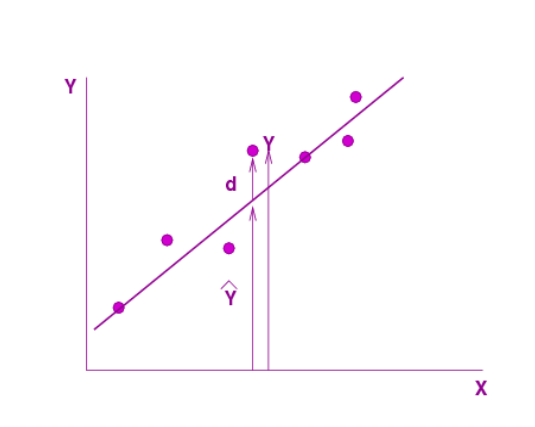
Fit a line whose equation is of the form $ \hat{Y} = a + b X $
Minimise $ L = \frac{1}{n} \sum_i d_i^2 = \frac{1}{n} \sum_i (Y_i − \hat{Y}_i )^2 $
- Find the expression for $ a^*$ and $b^*$ which optimise $ L $
Probabilistic Interpretation : Why L
Assumptions:
- Assume that $$ Y = \alpha + \beta X + \epsilon $$
where $$ \epsilon \sim N(0, \sigma^2) $$
- Write the expression for P[Y|X].
- Find the (conditional) MLE estimates of $ \alpha $ and $ \beta $ given n observations $ (x_1, y_1), (x_2, y_2), ... , (x_n, y_n) $.
[Pause after you equate $ \frac{\partial}{\partial \alpha} LL $ and $ \frac{\partial}{\partial \beta}LL$ to $ 0 $ ]
... To be continued in next class