Last Class:
MAP estimates
Beta distribution: Conjugate prior for a Bernoulli/Binomial likelihood.
LINEAR REGRESSION
Topics
$ MSE = Bias^2 + Variance $
Gauss Markov Theorem
Question 1
- Show $ E (b) = \beta $ under the assumption that $ y_i = \alpha + \beta x_i + \epsilon_i$ where $ \epsilon_i \sim N(0, \sigma^2)$. Thus show that least square estimators (a & b) are unbiased.
Relationship of bias and variance with MSE
Mean Square Error measure the "average" distance of the parameter estimate from its true value.
Question 2
Prove that:
$$ \begin{align} \operatorname{MSE_{\theta}}(\hat{\theta}) &= \operatorname{E}_{X|\theta} \left [(\hat{\theta}-\theta)^2 \right ] \\ &= \operatorname{Var}_{\theta}(\hat\theta)+ \operatorname{Bias}_{\theta}(\hat\theta)^2 \end{align} $$
[Hint Use the fact that $ Var(X) = E[X^2] - E[X]^2 $]
Gauss Markov Theorem
If:
- The expected average value of residuals is 0. ($ E(\epsilon_i ) = 0 $)
- The spread of residuals is constant and finite for all $ X_i (Var(\epsilon_i ) = \sigma^2 $ )
- There is no relationship amongst the residuals ( $ cov(\epsilon_i , \epsilon_j ) = 0 $)
- There is no relationship between the residuals and the $ X_i (cov(X_i , \epsilon_i ) = 0 $)
Then, least square estimates have lowest variance amongst all linear unbiased estimates.
Note: Our assumption that $ y_i = \alpha + \beta x_i + \epsilon_i$ where $ \epsilon_i \to N(0, \sigma^2)$ is a special case of the Gauss Markov theorem. (We additionally, assume that the $epsilon_i$ are normal distributed)
Proof:
Let the regression line be $ Y = b_{0} + b_{1}X$. Least square estimates of coefficients are given by: $$ b_{1} = \frac{\sum_{i}{(x_{i}-\bar{x})(y_{i}-\bar{y})}}{\sum_{i}{(x_{i}-\bar{x})^{2}}} = \sum_{i}{K_{i}Y_{i}} $$
where, $$ K_{i} = \frac{(x_{i}-\bar{x})}{\sum_{i}{(x_{i}-\bar{x})^{2}}} $$
and $$ Y_{i} = y_{i}-\bar{y} $$
And the other coefficient is given by, $$ b_{0} = \bar{y} - b_{1}\bar{x} $$
Now first calculate variance of $b_{1}$,
\begin{align*} \sigma^{2}(b_{1})= & \sigma^{2}(\sum_{i}{K_{i}Y_{i}}) \\ = & \sum_{i}{K_{i}^{2}\sigma^{2}(Y_{i})} .... (Why?)\\ = & \sigma^{2} * \sum_{i}{\frac{1}{(x_{i}-\bar{x})^{2}}} \end{align*}
Here $\sigma^{2}$ is the variance of each $Y_{i}$. \ Now consider another estimator of $\beta_{1}$ as $\hat{\beta_{1}}$.\ Let,
$$ \hat{\beta_{1}} = \sum_{i}{c_{i}y_{i}} $$
for some $c_{i}$.
Now consider expected value and variance of this estimator.
\begin{align*} E(\hat{\beta_{1}}) = & \sum_{i}{c_{i}E(y_{i})} \\ = & \sum_{i}{c_{i}E(\beta_{0} + \beta_{1}x_{i})} \\ = & \beta_{0}\sum_{i}{c_{i}} + \beta_{1}\sum_{i}{c_{i}x_{i}} \end{align*}
As $\hat{\beta_{1}}$ is an unbiased estimator, $E(\hat{\beta_{1}}) = \beta_{1}$ for generic values of $x_{i}$. \ So from above expression we can get conditions on $c_{i}$'s as\ $\sum_{i}{c_{i}}=0$ and \ $\sum_{i}{c_{i}x_{i}}=1$
Variance of the estimator is given by, \begin{align*} \sigma^{2}(\hat{\beta_{1}}) = & \sum_{i}{c_{i}\sigma^{2}(y_{i})} \\ = & \sigma^{2}\sum_{i}{c_{i}^{2}} \end{align*} Let $c_{i} = K_{i} + d_{i}$ for some $d_{i}$. Then we can write,
\begin{align*} \sigma^{2}(\hat{\beta_{1}}) = & \sigma^{2}*(\sum_{i}{( K_{i} + d_{i})^{2}}) \\ = & \sigma^{2}*(\sum_{i}{K_{i}^{2}} + \sum_{i}{d_{i}^{2}} + 2\sum_{i}{K_{i}d_{i}}) \\ = & \sigma^{2}\sum_{i}{K_{i}^{2}} + \sigma^{2}\sum_{i}{d_{i}^{2}} + 2\sigma^{2}\sum_{i}{K_{i}d_{i}} \\ = & \sigma^{2}(b_{1}) + \sigma^{2}\sum_{i}{d_{i}^{2}} + 2\sigma^{2}\sum_{i}{K_{i}d_{i}} .................. (\sigma^{2}\sum_{i}{K_{i}^{2}} = \sigma^{2}(b_{1})) \end{align*} Now consider the expression $\sum_{i}{K_{i}d_{i}}$.
\begin{align*} \sum_{i}{K_{i}d_{i}} = & \sum_{i}{K_{i}(c_{i} - K_{i})} \\ = & \sum_{i}{K_{i}c_{i}} - \sum_{i}{K_{i}^{2}} \\ = & \sum_{i}{c_{i}(\frac{(x_{i}-\bar{x})}{\sum_{i}{(x_{i}-\bar{x})^{2}}})} - \frac{1}{(x_{i}-\bar{x})^{2}} \\ = & \frac{\sum_{i}{c_{i}x_{i}} - \sum_{i}{c_{i}} - 1 }{\sum_{i}{(x_{i}-\bar{x})^{2}}} \end{align*} We know that $\sum_{i}{c_{i}x_{i}} = 1$ and $\sum_{i}{c_{i}} = 0$ as $\beta_{1}$ is an unbiased estimator (derived above). So substituting these values in above equation,
\begin{align*} \sum_{i}{K_{i}d_{i}} = & \frac{1 - 0 - 1}{\sum_{i}{(x_{i}-\bar{x})^{2}}} \\ = & 0 ........................................(*) \end{align*} Therefore we get,
\begin{align*} \sigma^{2}(\hat{\beta_{1}}) = & \sigma^{2}(b_{1}) + \sigma^{2}\sum_{i}{d_{i}^{2}} + 2*0 \\ = & \sigma^{2}(b_{1}) + \sigma^{2}\sum_{i}{d_{i}^{2}} \\ \geq & \sigma^{2}(b_{1}) \end{align*}
Thus, the least square estimate is the most efficient one amongst unbiased estimators.
Linear Regression: Summary
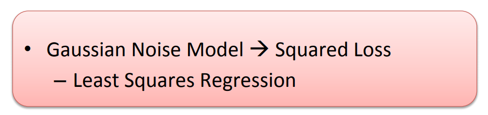
- Minimizing the Mean squared loss function, L is the same as minimizing the (conditional) negative log likelihood (Maximizing the likelihood) under the assumption that $ Y|X \sim \alpha + \beta X + \epsilon ; \quad \epsilon \sim N(0, \sigma^2) $
- Thus $$ b = \frac{\sum{x'_i y'_i}}{\sum{x'_i}^2} = \frac{sample \; covariance \; between \; x \; and \; y} {sample \; variance \; of \; x} $$
$$ a = \bar{y} - b \bar{x} $$ correspond to MLE estimates with the above assumption
- Both the above estimates are unbiased.
- The Gauss Markow theorem states that amongst unbiased estimates, the above estimates have the least variance and are thus the most efficient ones. BLUE - Best Linear Unbiased Estimator