Probabilistic Graphical Models
Introduction
Generative Models v/s Discriminative models:
- Generative: Model the joint distribution of all the random variables (X) i.e P(X).
- Discriminative: Model the conditional probability of some of the variables (say Y), given other ones (say X) i.e P(Y|X)
- Q. Suppose $ | Y | = n $ and $ | X | = m $. Assume all the random variables are binary. How many parameters would you have to learn if you want to build a:
- Discriminative model?
- Generative model?
- You can obtain a discriminative model from a generative one.
- Discriminative models involve lesser complexity than the Generative ones.
Why Probabilistic Models?
- Probabilistic models capture the uncertainty in the result as well.
- Some people believe that there's an inherent stochasticity in nature. So, everything is probabilistic.
- Probability theory has been well studied. Can utilize the Statistical learning toolbox.
Why Graph Representation?
- Sparse Parametrization
- Efficient Algorithms to reason from the data.
Two types of models:
- Bayesian Networks: Directed Models
- Markov Networks: Undirected Models
Where have these been used?
- Bayesian Networks: Medical Diagonsis
- Markov Networks: Image Segmentation
Quiz
Q1
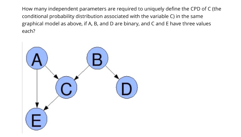
Q2.
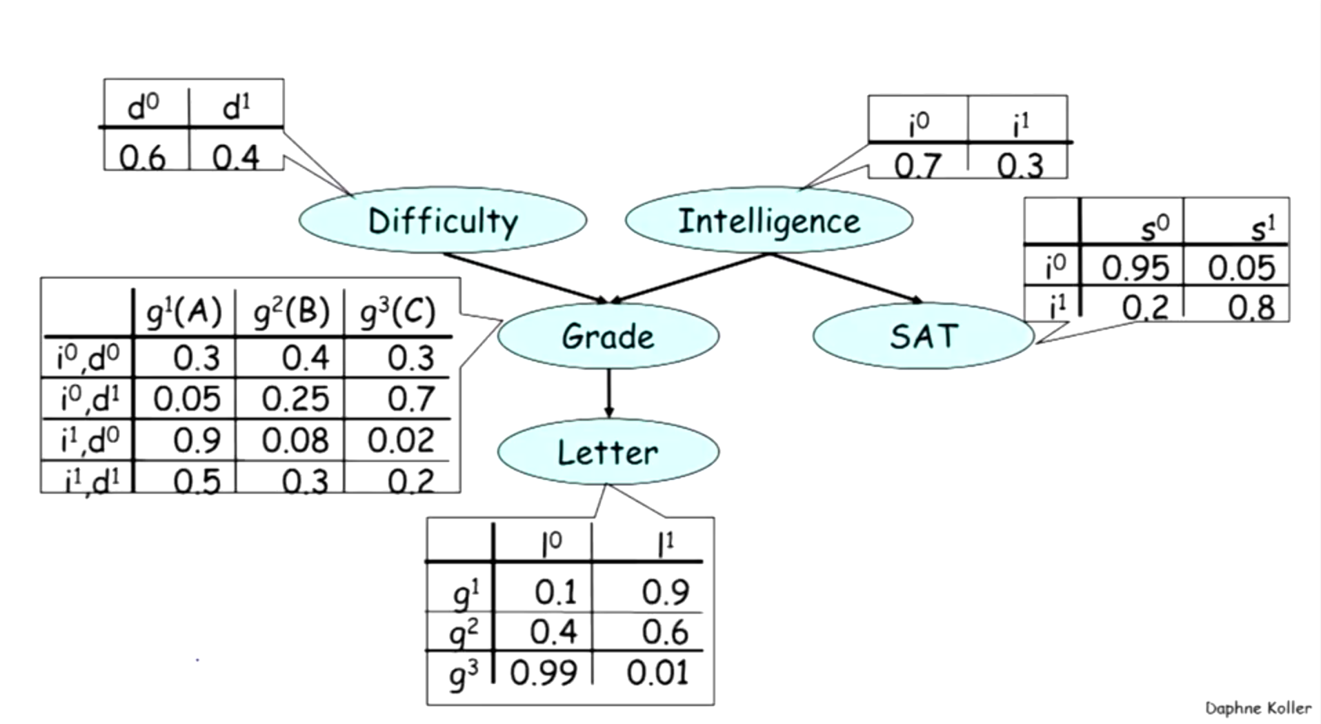
Calculate:
$ P(d^0, i^1, g^3, s^1, l^1) $
$ P(d^0, i^1,l^1) $
$ P(G | i^0, d^0) $
$ P(G | i^0) $
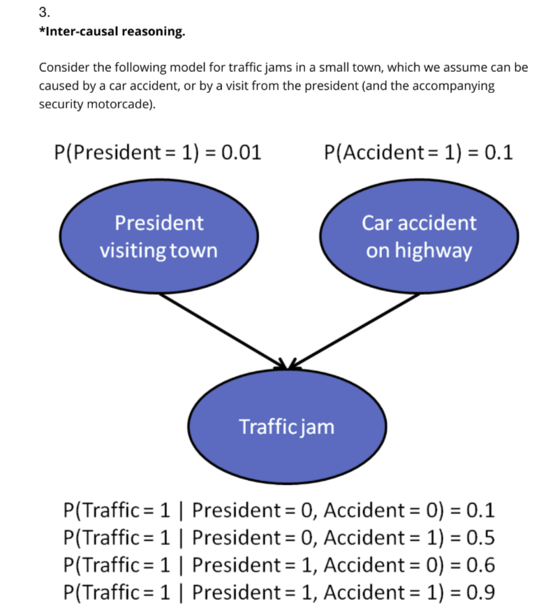
Q3 Calculate P(Accident = 1|President = 1) and P(Accident = 1| Traffic=1, President = 1)
Learning Bayesian Networks
- Chapter 6 - Paramaeter learning: Binary Variables from Learning Bayesian Networks.
Structure learning v/s parameter learning
- Two types of learning: Structure and Parameter learning. Both of them can be learnt from data.
- Linear Regression. The use of regularization as a means to achieve structure learning and parameter learning simultaneously.
- Here we'll use that we have structure given to us. All we need to do is learn the Parameters.
Beta distribution
- $$ \Gamma(x+1)=\int_{0}^{\infty}t^{x}e^{-t} $$
- $$ \Gamma(x+1)=x \; \Gamma(x) $$
- $$ B(x,y)=\int_{0}^{1}t^{x-1}(1-t)^{y-1} dt = \frac{\Gamma(x) \; \Gamma(y)}{\Gamma(x+y)} $$
- $$ Beta(x \; | \; \alpha, \beta) = \frac{x^{\alpha-1} \; \; (1-x)^{ \; \beta-1} }{ B(\alpha,\beta) } $$
Coin: Single node Bayesian Net
- You have a coin. Assume that it is a biased coin and $ Side \sim Bernoulli(f). $
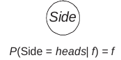
- Your task is to learn $ f $. Let $ F $ be a random variable for the parameter $ f $. You have certain beliefs about the value of parameter $ f $ and you encode it in the prior $ F \sim Beta(f; \alpha, \beta) $.
- Q. Suppose your Prior is $ F \sim Beta(f; a, b) $. What is $ P(Side=heads) $ ?
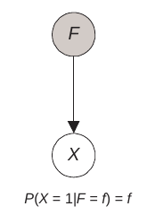
Theorem 6.1
Suppose $ X $ is a random variable with two values 0 and 1, $ F $ is another random variable such that
$$ P(X = 1 | F = f) = f $$
Then,
$$ P(X = 1) = E(F) $$
Now in order to learn the parameter, you let's model $ F $ along with the our variable $ X $. This is called as the Augmented Bayesian Network representation of our earlier Bayesian Net.
Let's $ F $ follow the density function $ \rho $ which is called the prior density function of the parameters.
Now by the Bayes' rule we have $$ P(F=f\;|\;D=d) = \frac{P(D=d \;|\; F=f) \rho (f)} {P(D=d)} $$ In this way, we'll learn the distribution of $ F $ from the data.
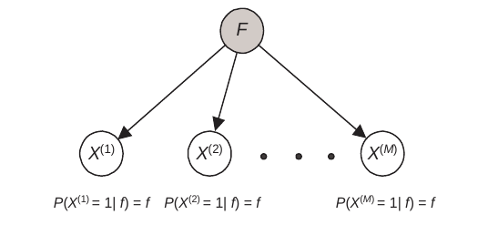
Definition 6.2
Suppose
We have a set of random variables (or random vectors) $ D = { X^{(1)} , X^{(2)} , . . . X^{(M)} } $ such that each $ X^{(h)} $ has the same space.
There is a random variable $ F $ with density function $ \rho $ such that the $X^{(h)}$ s are I.I.D. for all values $ f $ of $ F $.
Then $ D $ is called a sample of size $ M $ with parameter $ F $.
Given a sample, the density function $ \rho $ is called the prior density function of the parameters relative to the sample. It represents our prior belief concerning the unknown parameters.
Given a sample, the marginal distribution of each $ X^{(h)} $ is the same. This distribution is called the prior distribution relative to the sample. It represents our prior belief concerning each trial.
Definition 6.3
Suppose we have a sample of size $ M $ such that
- each $ X^{(h)} $ has space $ {0, 1} $;
- $ F $ has space $ [0, 1] $, and for $ 1 ≤ h ≤ M \quad P (X^{(h)} = 1| f) = f $.
Then $D$ is called a binomial sample of size $M$ with parameter $F$.
Theorem 6.2
Suppose
- $D$ is a binomial sample of size $M$ with parameter $F$.
- We have a set of values $d = {x^{(1)} , x^{(2)} , . . . x^{(M)}}$ of the variables in $D$ (The set $d$ is called our data set (or simply data)).
- $s$ is the number of variables in $d$ equal to $1$.
- $t$ is the number of variables in $d$ equal to $0$.
Then $ P(d) = E(F^s (1 − F)^t) $.
Proof : Marginalization: $$ P(D = d) = \int_0^1 P(D=d \;|\; F = f) \rho(F = f) df $$
Corollary 6.2
If the conditions in Theorem 6.2 hold, and $F$ has a beta distribution with parameters $ a, b, N = a + b$, then,
$$ P(d) = \frac{\Gamma (N)}{\Gamma(N + M)} \frac{\Gamma(a + s) \Gamma (b + t)}{\Gamma(a) \Gamma(b)} $$
Proof: Application of Lemma 6.4
Lemma 6.4
Suppose $F$ has a beta distribution with parameters $a, b$ and $ N = a + b$. $s$ and $t$ are two integers ≥ 0, and $M = s + t$. Then
$$ E[F^s \; [1 − F]^t] = \frac{\Gamma (N)}{\Gamma(N + M)} \frac{\Gamma(a + s) \Gamma (b + t)}{\Gamma(a) \Gamma(b)} $$
Lemma 6.5
Suppose $F$ has a beta distribution with parameters $a, b$ and $ N = a + b$. $s$ and $t$ are two integers ≥ 0, and $M = s + t$. Then
$$\frac{f^s (1 − f)^t \rho(f)}{E(F^s [1 − F]^t )} = Beta(f ; a + s, b + t) $$
Theorem 6.3
If the conditions in Theorem 6.2 hold, then $$ ρ(f|d) = \frac{f^s (1 − f )^t ρ(f)}{E(F^s[1 − F ]^t)} $$
where $\rho(f|d) $ denotes the density function of $F$ conditional on $D = d$.
Conclusion:
Corollary 6.3
Suppose the conditions in Theorem 6.2 hold, and F has a $ Beta $ distribution with parameters $a, b$ and $ N = a + b$. That is, $$ ρ(f) = Beta(f ; a, b) $$
Then, $$ ρ(f |d) = beta(f ; a + s, b + t) $$
Theorem 6.4
Suppose the conditions in Theorem 6.2 hold, and we create a binomial sample of size $M + 1$ by adding another variable $X^{(M+1)} $ . Then if $ D $ is the binomial sample of size $ M $, the updated distribution relative to the sample and data $ d $ is given by
$$P(X^{(M +1)} = 1| d) = E(F |d) $$
Corollary 6.4
If the conditions in Theorem 6.4 hold and F has a beta distribution with parameters $a, b$ and N = a + b, then
$$ P(X^{(M +1)} = 1| d) = \frac{a + s}{N + M} = \frac{a + s} {a + s + b + t} $$
Next class
- Marginalization (Some Problems)
- Connections and building blocks of Bayesian Networks
- Conditional Independences: d - Separation
- Multinomial distribution